Kalman Filter

Using the Kalman Filter on IOT-sensor temperature data in Python

I started looking into the Kalman Filter for a separate project on cleaning sensor data and found that there was limited online Python resources, so I’d like to use this page to add on to the existing and provide my code in case someone out there can find it useful. I’m also happy to hear from others if the way I ended up using the filter was completely incorrect.

Since I am not well versed in the Kalman Filter, I will not be going into the mathematical definition, but there is a wealth of information online. I will be using the Kalman Filter in a single dimension solution (i.e. not calculating velocity), for temperature measurement readings from an IOT sensor. The csv file was downloaded from Kaggle and can be found here.


Importing libraries

import pandas as pd
import plotly as py
import plotly.express as px
import plotly.figure_factory as ff
import numpy as np
import scipy.stats as stats
import matplotlib.pyplot as plt
import statsmodels

from itertools import compress
from math import *
from sklearn.metrics import mean_squared_error, r2_score, mean_absolute_error
from sklearn.model_selection import train_test_split
from pykalman import KalmanFilter

from scipy import interpolate
from sklearn import datasets, linear_model
from sklearn.model_selection import train_test_split
from sklearn.metrics import mean_squared_error
from math import sqrt
from statsmodels.tsa.api import ExponentialSmoothing, SimpleExpSmoothing, Holt
from plotly.offline import init_notebook_mode, plot, iplot
init_notebook_mode(connected=True)

Data describe

The data provided had both an inside and outside data sensor, so I decided to split the original dataset into two based on this Boolean value.

Summary:

  1. Total data pts = 97606, 8733 inside, 22605 outside

  2. Inside mean = 30.67, outside mean = 39.51

  3. Inside min = 21, outside min = 24

  4. Inside max = 41, outside max = 51

df = pd.read_csv (r'C:\Users.... (enter your file path)
df_out = df[(df['out/in']=='Out')]
df_in = df[(df['out/in']=='In')]

# Inside Sensor data set
temp_in = pd.DataFrame(df_in, columns=['noted_date', 'temp'])
temp_in = temp_in.groupby(['noted_date']).mean()
temp_in.reset_index(inplace=True)
temp_in['temp_inside'] = temp_in['temp']
del temp_in['temp']
print (temp_in.describe())

# Outside Sensor data set
temp_out = pd.DataFrame(df_out, columns=['noted_date', 'temp'])
temp_out = temp_out.groupby(['noted_date']).mean()
temp_out.reset_index(inplace=True)
temp_out['temp_outside'] = temp_out['temp']
del temp_out['temp']
print (temp_out.describe())
Inside temp.png

Inside temp

Inside Temp over time

Outside temp.png

Outside temp

Outside temp over time


Kalman Filter Python code

The below is the Kalman Filter model I used on the Inside temperature data from above. I did break this table into a train and test, but will not be covering that portion of the code here.

# Kalman Filter model
# using the Kalman Filter to clean the Inside IOT sensor 
measurements = np.asarray(temp_in)

kf = KalmanFilter(transition_matrices=[1],
                  observation_matrices=[1],
                  initial_state_mean=measurements[0,1],
                  initial_state_covariance=1,
                  observation_covariance=5,
                  transition_covariance=1) 
state_means, state_covariances = kf.filter(measurements[:,1]) 
state_std = np.sqrt(state_covariances[:,0]) 

plt.figure(figsize=(12, 8))
plt.plot(measurements[10:,0], measurements[10:,1], '-b', label='Data') 
plt.plot(measurements[10:,0], state_means[10:,0], '-r', label='Kalman-filter 5') 
plt.legend(loc='upper left') 
plt.show()

kalmandf = pd.DataFrame(state_means, columns=['temp_inside_KF'], index=temp_in.index)

temp_kalman = pd.concat([temp_in,kalmandf], axis=1)
print(temp_kalman.head(10))

temp_kalman.drop(temp_kalman.head(10).index, inplace=True)

print('')
print ('--Kalman Filter--'*5)
print(model_eval(temp_kalman['temp_inside'],temp_kalman['temp_inside_KF']))
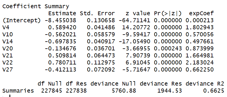
Inside Kalman.png

Model Performance

Mean Absolute Error: 0.24 Mean Squared Error: 30.375 R2 Score: 0.953 Root Mean Squared Error: 0.504 Mean absolute percentage error: 0.806 Scaled Mean absolute percentage error: 0.802 Mean forecast error: 30.368 Normalised mean squared error: 0.047 Theil_u_statistic: 0.001

Logistic Regression

Conclusions up front

Reduced the model to 7 variables to predict credit fraud risk. Variables V4, V21, and V22 are roughly 2x increase to the likelihood of credit card fraud. Variables V10, V14, and V27 roughly reduce the likelihood of credit card fraud by half.

This is a logistic regression analysis on Credit Card Fraud Detection, using a dataset from Kaggle.com

creditcard.csv > glimpse(CCFraud) Rows: 284,807 Columns: 31

Target = “Class”, a binomial target where 0=not fraud, 1 = fraud.

30 Variables include Time, V1 thru V28, and Amount. All variables are numeric, and variables starting with ‘V’ lack description due to data confidentiality.

Libraries loaded: tidyverse, GGally, ROCR, caret, funModeling, skimr

Credit Card Fraud (Class = 1) has an average V4 of ~4, whereas non fraudulent credit card charges (Class = 0) have an average V4 of 0.

A majority of variables exhibit normal distribution and do not require the log transformation - it is likely they have been pre-normalized for this exercise

V17, V14, V12, V10, and V16 exhibit negative correlation coefficients above abs(0.2)

Summary


First Model: kitchen sink approach

Using all variables to run the first model shows promising results but likely overfit (too many variables). FirstModel <- glm(Class ~ Amount + Time + V1 + V2 + V3 + V4 + V5 + V6 + V7 + V8 + V9 + V10 + V11 + V12 + V13 + V14 + V15 + V16 + V17 + V18 + V19 + V20 + V21 + V22 + V23 + V24 + V25 + V26 + V27 + V28,family = binomial(logit), data = CCFTrain)

Quality

  • Res Deviance: 1826.58

  • Null Deviance: 5760.88

  • Deviance Pseudo R²: 68.3%

Accuracy

  • Threshold: 0.5

  • Recall: 61.89%

  • Precision: 88.32%

Summary

  • Poor performance despite the good quality metrics, there are many variables with no significance that can likely be removed.

  • We need to evaluate 5% of the population with high probability of fraud to capture 80% of the fraud cases

  • Variables V4 & V22 increases the likelihood of CC Fraud by 2x

  • V10 & V27 decrease the likelihood of CC Fraud


Second Model : running the stepwise function

The stepwise function returns 16 variables out of the 30 with similar results to the First Model. This function removes variables one by one (likely ones with no significance (p<0.05)) and reruns a new model each round to land at the ‘optimized' model performance.

Quality

  • Res Deviance: 1834.35

  • Null Deviance: 5760.88

  • Deviance Pseudo R²: 68.2%

Accuracy

  • Threshold: 0.5

  • Recall: 61.38%

  • Precision: 88.24%

Summary

  • This model is much improved by the reduction of non significant variables. But there is potential to continue removal of variables with smaller impact on detecting CC Fraud - those with coeff ~1.

  • We need to evaluate 5% of the population with high probability of fraud to capture 80% of the fraud cases

  • Variables V4 & V22 increases the likelihood of CC Fraud by 2x

  • V10 & V27 decrease the likelihood of CC Fraud


Third Model: self selection

Based on the outcome above from the stepwise function, we can run a third model, reducing the variable count to 7, roughly half of the above model and still retain decent results. I selected variables with coefficients further from 1:

ThirdModel <- glm(Class ~ V4 + V10 + V14 + V20 + V21 + V22 + V27, family = binomial(logit), data = CCFTrain)

Quality

  • Res Deviance: 1944.53

  • Null Deviance: 5760.88

  • Deviance Pseudo R²: 66.3%

Accuracy

  • Threshold: 0.5

  • Recall: 58.31%

  • Precision: 86.69%

Summary

  • I lost 3% of recall and ~2% of precision by cutting the variable inputs by half, so maybe not a major loss for a model that shows more clearly which variables are the most important.

  • We need to evaluate 4% of the population with high probability of fraud to capture 80% of the fraud cases

  • Variables V4 & V22 increases the likelihood of CC Fraud by 2x

  • V10, 14 & V27 decrease the likelihood of CC Fraud


Finding the right Threshold

In the previous models I was using a default Threshold of 0.5. The Threshold is the value above which the data point will be considered positive (or CC Fraud detected) on a scale between 0 and 1. Recall (aka True Positives of CC Fraud) measures the amount of true positives divided by true positives + false negatives (aka the total observed amount of CC Fraud). Precision measures the amount of true positives divided by trust positives + false positives. Accuracy measures the overall correct predictions of the model divided by the total data points. Calculating the F1 Score can determine the best threshold for balance between recall and precision.

  • Threshold = 0.6, F1 Score = 0.68

  • Threshold = 0.5, F1 Score = 0.70

  • Threshold = 0.4, F1 Score = 0.69

Based on the above, the threshold of 0.5 is actually the best suited line to draw in the sand to push the output into either 1=Fraud, or 0=No Fraud.


Checking the model with TEST data

Running the test data (I split the original data between 80% train, and 20% test) through the third model to see how well the model performs with a new set of data. By testing the model against the test data we can confirm that the model is consistent with different data points.

Accuracy

  • Threshold: 0.5

  • Recall: 64.36%

  • Precision: 82.28%

Summary

Some minor moves in recall and precision, but I believe the moves are not enough to justify that this model should be thrown away.